SCHEDULE FORECASTING MADE SIMPLE
I do not intend to conduct extensive review of forecasting and trend analysis methods. Those are widely available in literature. I intend to present to busy practitioners like myself, a simple, easy-to-use, and reliable forecasting method that they can use, without having to be techie or math whiz to do so!
The method assumes what John Chambers et al, in their essay “How to Choose the Right Forecasting Technique”, call ‘A-Future-Like-Past’. That is, existing patterns are expected to continue into the future. They are of the opinion that “this assumption is more likely to be correct over the short term than it is over the long term, and therefore, these techniques deliver ‘reasonably accurate forecasts’ for the immediate future but do quite poorly further into the future (unless the data patterns are extraordinarily stable).” However, I have used the method to forecast project completion with satisfactory results, 9 months ahead of time. Therefore, the definition of short term or long term is open to argument.
In addition, each project team needs to determine what ‘reasonably accurate forecast’ is for them. From a practitioner’s point of view, stakeholders are rarely concerned with the project being completed on Wednesday afternoon, or the following Thursday morning. For most projects, a slippage of 1.5% may not raise red flags; the project team usually thinks it can manage. However, for a one-year construction project, that represents a delay of almost one week. Therefore, if your simplified forecasting method shows that the project is likely to be delayed by one week, if present trends continue, then that is enough to put the project leadership at alert. That is a lot better than the usual, “we’re just 1.5% behind and we’re confident that we’ll deliver on time.”
I would like to give a bit of theoretical background before delving into the technique itself.
This simplified forecasting method relies on the fact that the S-Curve (a winding path), or its segment, can be replaced with an equivalent straight line. In other words, we attempt to replace the growth curve with an equivalent linear function. This is not a novel idea; you may check here for another application of the principle (https://electronics.stackexchange.com/questions/1983/correcting-for-non-linear-brightness-in-leds-when-using-pwm).
Experience shows that, for most project schedule or completion forecasting purposes, this is adequate. John Chambers and his partners have advised that if the forecaster can readily apply one technique of acceptable accuracy, he or she should not try to “gold plate” by using a more advanced technique that offers potentially greater accuracy but requires nonexistent information or information that is costly to obtain. I would also like to add, that is cumbersome to use. The reality is that the more cumbersome the method is the more unlikely it is that the team will use it.
The S-Curve, which is the standard and most common means of monitoring project progress, is commonly represented by the equation below.
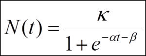
Those who have no interest in this complex equation need not bother. The main purpose of this essay is to demonstrate that we do not need complex mathematics to deliver desired result.
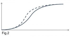
The graphics below (Fig. 1) presents the standard form of the S-Curve. Fig.2 show both planned progress (in continuous line) and actual progress (in dotted line). The vertical axis represents progress while the horizontal axis represents time.
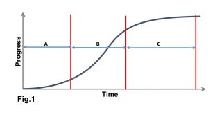
The shape of the curve shows that there is a slow start at the beginning of the project (Section A, Fig. 1), where the project team is being mobilized, and getting familiar with project processes, etc. Then there is rapid progress as the project picks up pace (Section B). Finally, another slow progress as the project winds down and project resources are gradually demobilized (Section C).
Historical performance data is used to predict the future, typically Milestone Completion Date (MCD) or Project Completion Date (PCD). The fundamental assumption here, as already mentioned above, is that we expect current trends to persist. Therefore, the project must have a relatively stable historical pattern for the method to deliver reliable results. So, this should not be used too early in the project.
I guess all project control persons would need to be engineering or mathematics graduates to be able to use the S-curve equation to do that. Even at that, the rigor required and the accuracy obtained may not justify the effort.
Thankfully, an alternative method exists that is simple and delivers satisfactory results repeatedly, in my experience. In addition, because forecasting is not a one-off exercise in the life of a project, the simpler the forecasting method, the better, and the more likely that project control personnel will actually use it.
A common wisdom in project control is that a project control system should not be more rigorous or expensive to implement than the result it delivers. That makes sense!
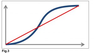
The logic behind the simplified method is simply trying to find the time it would take to travel steadily along a straight line, defined by historical performance and extrapolated into the future, from the beginning of the project to the end, rather than follow the winding path of the S-Curve. After all, the destination is our objective, whether it is the MCD or PCD.
This method replaces the S-Curve with a corresponding straight line (Fig. 3), thus turning the complex equation into a linear function that simplifies forecasting. Each point on this straight line is the historical average cumulative productivity up to that point.
The simplified forecasting method is a two-step process:
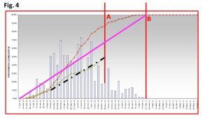
Step 1: Replace Actual Progress with an equivalent straight line (the bold, black dotted line in Fig. 4). This replaces the varied progress per time with an equivalent constant progress represented by average cumulative progress over the period, up to Data Date (point A). The more stable the pattern of past performance up to this point, the better the prediction of the future.
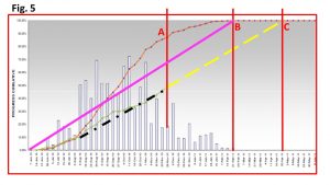
Step 2: Extrapolate, or extend or project this into the future. This is based on the assumption that the future will be like the past. The bold, yellow, dotted line represents this. After all, the forecast is simply what might happen if current trend persists! This shows a new forecast completion date (MCD or PCD), point C in Fig. 5.
To Summarize:
- The original Planned or Target S-curve is shown in Fig 5, terminating at point B, representing project completion at 100% progress.
- The Planned S-curve may be represented by an equivalent straight line showing steady equal periodic progress from start to completion – at some points productivity is higher than S-curve Planned, and at other times lower.
- The actual progress is shown in green, and is significantly behind plan. The heavy, dotted, black line represents a steady, constant periodic progress, or average periodic progress over time.
- The heavy, dashed, yellow line represents the forecast of this trend into the future. It demonstrates that the completion date will end up at point C instead of B, representing about two months delay.
With this, we are in a position to say, mathematically:
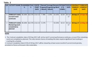
- It takes so many days to produce 1% progress. Therefore, it will take so many days to complete the remaining works. For instance, if it takes 5 days to achieve 1% progress and remaining works is 30%, then we can safely conclude that it would take 5*30 = 150 days, or 5 months from today, to complete the project, if current trend persists. However, if unforeseen negative risks materialize then the project may suffer further delay.
I will now demonstrate this by an example.
Step 1:
Compute the average cumulative progress for the period – per day, week or month. This is shown in Progress Statistics (Table 1) below.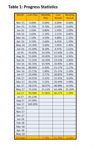
Step 2:
Use this to calculate the forecast completion date as shown in the figure Forecast Completion Dates (Table 2) below.
Step 3:
Draw conclusions to guide the project leadership concerning the basis of your forecast and what to expect. This, to me, is the most useful part of the exercise, and the purpose for forecasting – to advise the team what to expect, and what needs to be done to change things. This is where you bring all the known issues that cannot be modeled, into consideration.
In conclusion, I have shown that the process of forecasting project completion dates based on historical actual performance can be simplified if the s-curve, or its segment, is replaced by an equivalent straight line. The more stable the historical pattern, the more reliable the result. Forecasting becomes a simple matter of extrapolation into the future. In my experience, this has yielded satisfactory results repeatedly.
The notes or conclusions you draw are of utmost importance. For instance, if the forecast completion date for a construction project puts the completion date in the rainy or monsoon season, it should be noted because it is likely to cause further delay.
I hope that this helps our teeming population of young and upcoming planning engineers.


